Installation
When you first purchase DICOM 3D from our store, you will be provided with 3 Download options:
- MacOS Apple Silicon: This provides an installer compatible with Mac devices with M1 chips or newer, i.e. Mac devices from 2020 and newer. Don't use this installer if your device contains an Intel processor.
- MacOS Universal: This provides an installer compatible with Mac devices with either Intel or Apple Silicon chips, hence the name Universal. This installer will provide a DICOM 3D application compatible with Intel chips. If you purchased your device before 2020, use this option. If your device has an M chip, use the Apple Silicon installer.
- Windows Installer: This provides a link to the Microsoft Store DICOM 3D Page, where the Windows version of this application is available for download.
For Mac Devices, in order to check what kind of processor your computer has, click the Apple Icon at the top left of your screen, followed by About This Mac. Here, MacOS will provide you with a summary of your device's specifications.
On MacOS, once downloaded, open DICOM-3D.pkg and follow the steps provided by the installer.
On Windows, on the DICOM 3D Microsoft Store Page, select the Install option, and Windows will handle the rest.
Licensing
If you purchased DICOM 3D on our store, when you first start the application, you will be presented with two options. Either Start Free Trial, or Enter License Key.
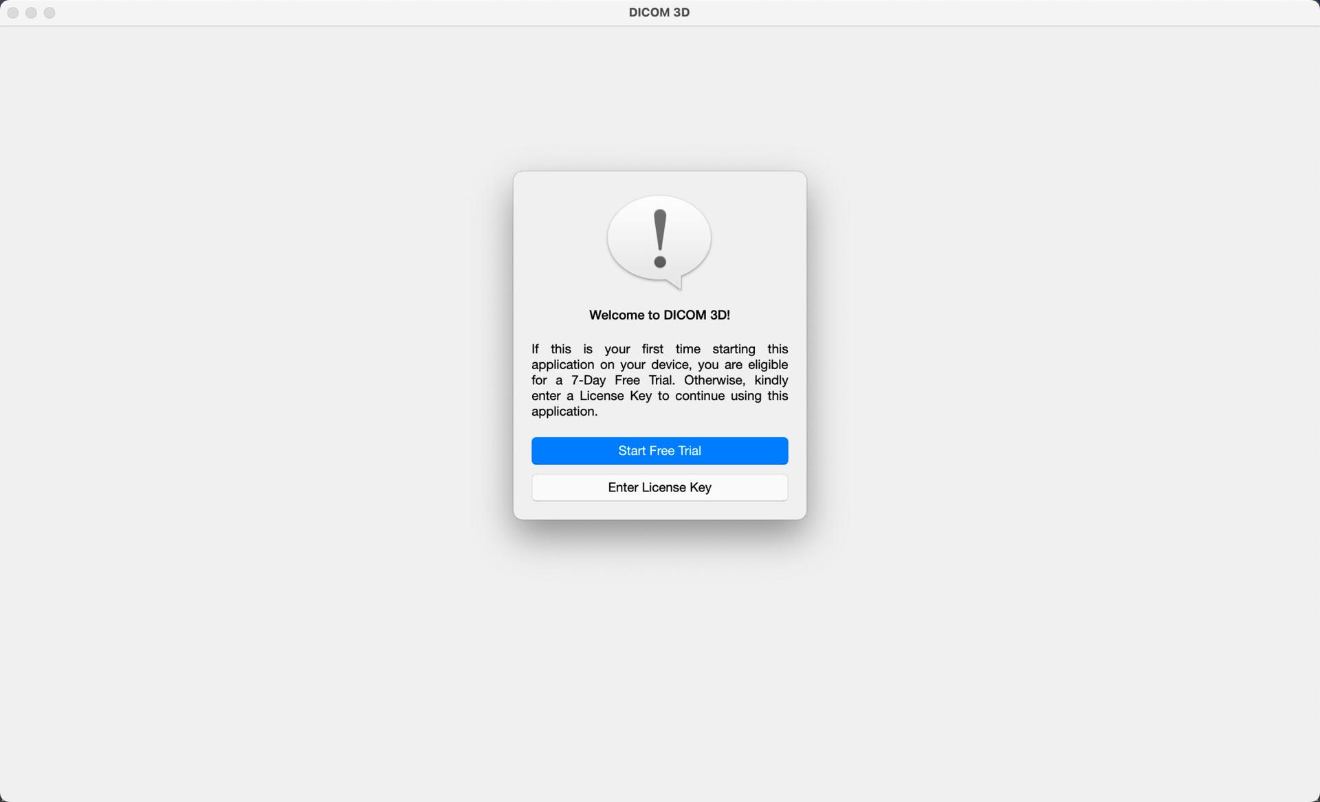
Start Free Trial: DICOM 3D offers new users a free 7-Day Trial of the application, before a license is required. This gives new users time to acquaint themselves with the application, and its features, before deciding on whether to make the purchase. This option can only be used once on a device, and the countdown begins as soon as you select Start Free Trial.
Enter License Key: If you have already completed a 7-Day free trial, the application will require a License Key for continued use. License Keys are available for purchase on our store here. You have an option of buying an Annual License or a Lifetime License. Once purchased, the license key will be included in an email confirming your order. If you created an account during the purchase process, or have an account already, all purchased keys are also available on the Downloads section of your Account's Dashboard, available here. After purchase, simply copy and paste the license key exactly as it is, onto an input provided in the application when prompted. Once verified, the license will be saved on your device, and you will not have to enter it again.
Navigation
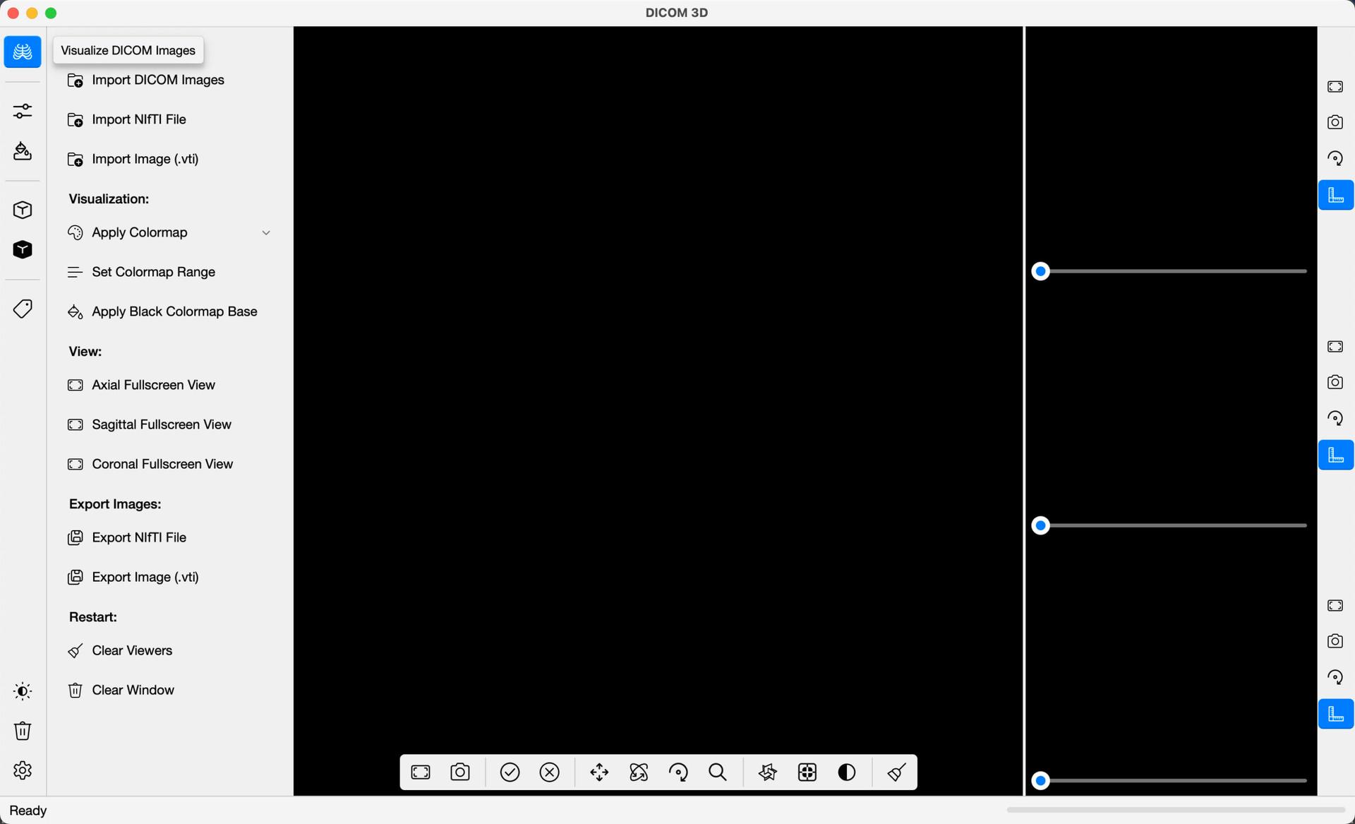
DICOM 3D has a navigation bar on the left from which you can launch the main features of the application. For each of the listed options below, when selected, a command bar is brought to view at the of the window, with the respective functions:
- Visualize DICOM Images
- Threshold Segmentation
- Watershed Segmentation
- 3D Reconstruction
- 3D Volume Rendering
Select DICOM Tags to bring up a table that comprises a comprehensive list of DICOM Tags. When a series of DICOM Images is imported, this table is populated with the corresponding Tag Values.
Select Toggle Light/Dark Mode , to change the theme of the application. By default, the application will match your device's theme. However, you can override this by manually selecting your preferred theme.
Select Delete Imported Study & Clear All Viewers , to delete all imported images and generated models.
Select Settings to bring up a list of preferences that you can customize to personalize DICOM 3D to your liking.
Import DICOM Images
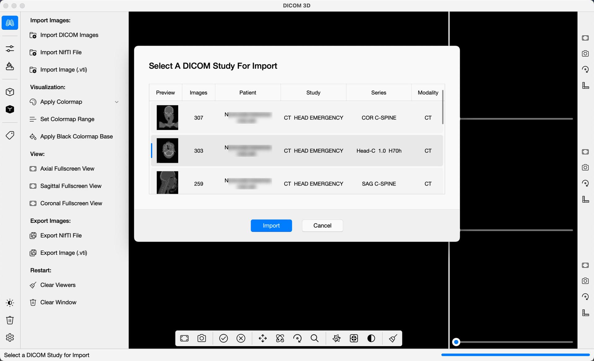
DICOM Images can be imported in one of two ways. Either, on the command bar, select Import DICOM Images , or from the menu bar, select, File -> Import DICOM Images . Once selected, a dialog box will open, allowing you to select the location of the DICOM Images in your computer. Select the folder containing the images. The application will sort the Images into their respective series, and give you a preview of each, as illustrated in the image below. A summary of each series including the number of images, patient names, study description, series description and modality are provided. Select the row in the table containing the series you wish to import, and Import.
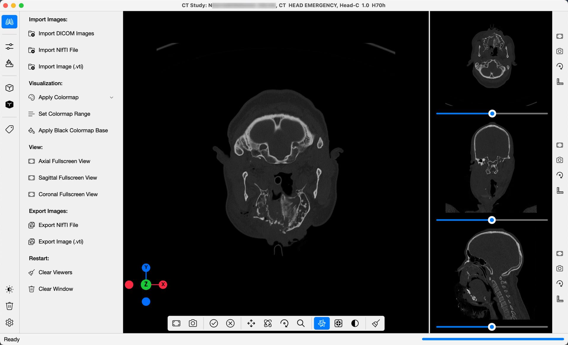
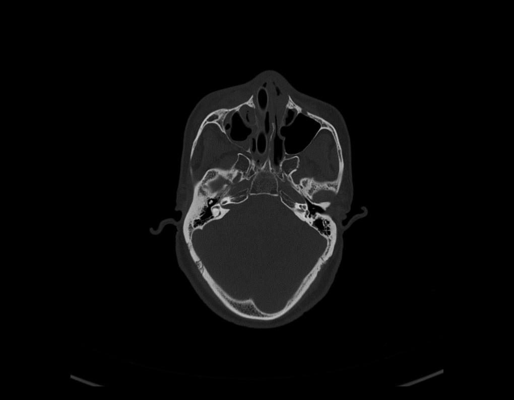
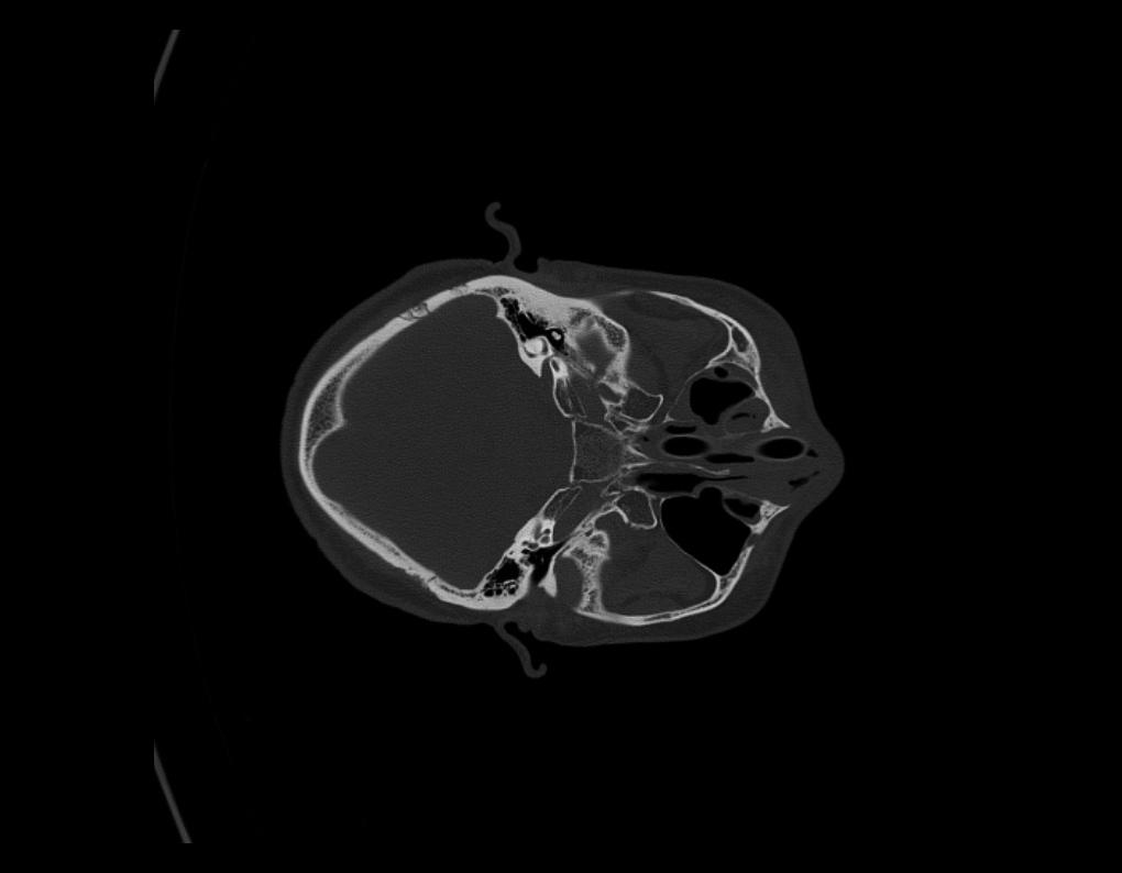
Upon importation, slices in each of the Axial, Sagittal & Coronal Orientations will be loaded into each of the three 2D Views Stacked to the right. The images will be initially loaded in grayscale. Use the slider below each view to scroll through all the images in the Series, in that orientation.
In the centre, you will find each slice loaded into the 3D View. Rotate the images to see each slice in 3D Space. As you scroll through the slices, they will be updated in the 3D View in real-time, giving you a more complete perspective of the Medical Images. These 3D slices can be toggled on/off at any time using the Show/Hide 3D DICOM Slices button, highlighted in blue below the 3D view.
To the right of each 2D View, you will find a set of four buttons. When clicked, each button offers a different way of interacting with the 2D Slices, as listed below:
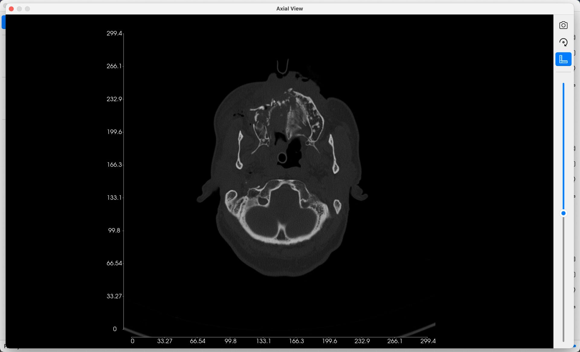
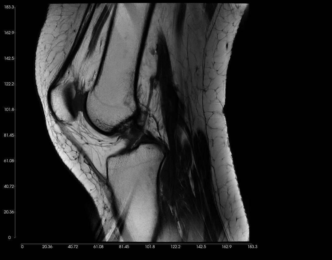
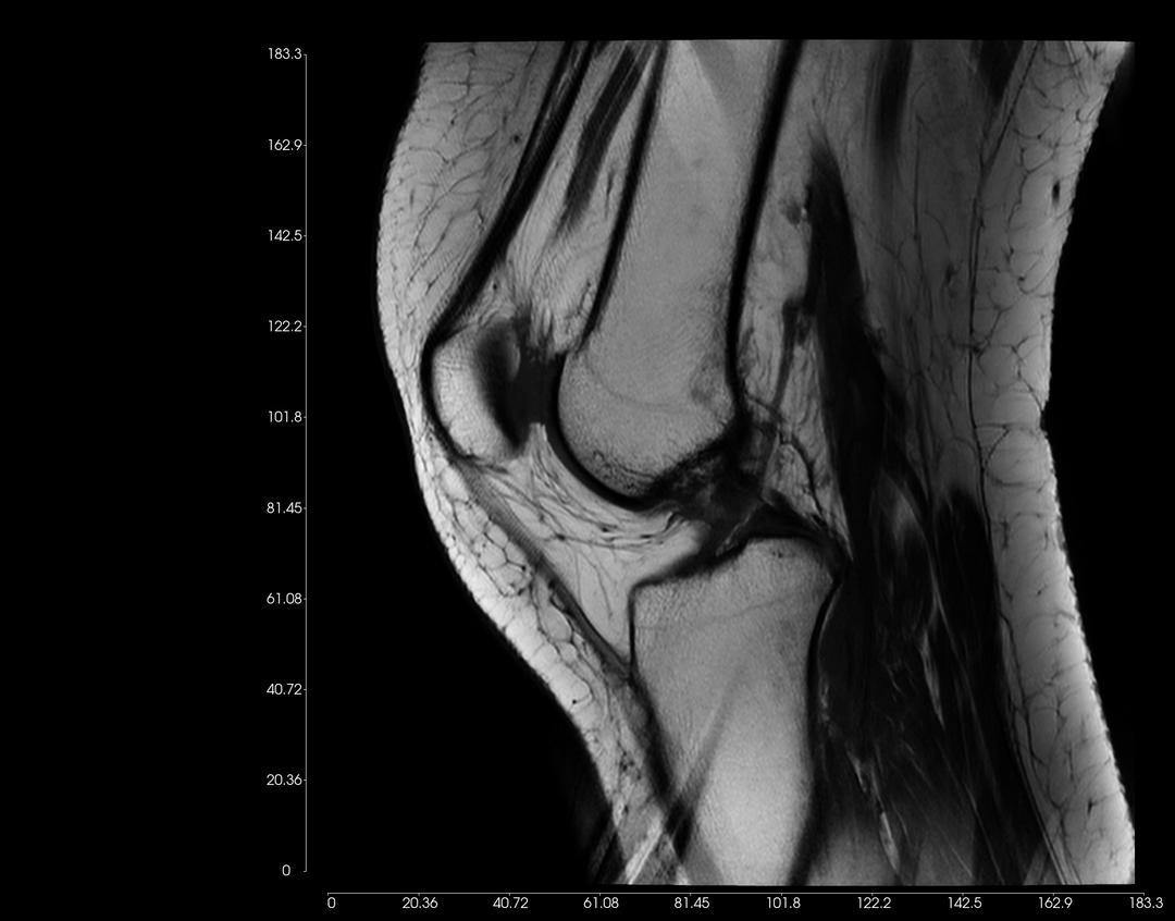
- Extend View To Fullscreen: Bring up a fullscreen display of the 2D View, as presented in the image below.
- Export Screenshot of Slice: Save a PNG/JPEG Image of the 2D Slice at a location of your choice.
- Rotate Slice by 90°: As the hint suggests, rotate the respective slice by 90°. This can be useful in rare instances where images are loaded in the wrong orientation.
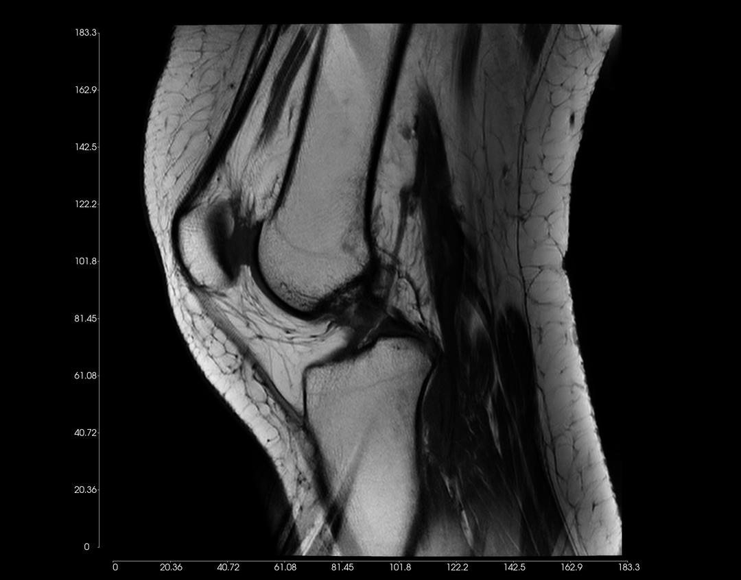
- Show/Hide Measurement Axes: Toggle on/off an accurate axes measurement in millimetres, displayed on each slice.
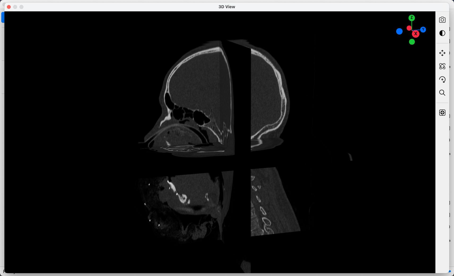
Similar to the 2D Views, select the Extend View of 3D Window button, found in the toolset below the 3D View, to display 3D Models in fullscreen as in the example below. Interact with the 3D Models as you normally would.
Once 3D Models are loaded into the 3D View, a 3D-coordinate widget will also be added, that gives you an indication of the orientation of the current view. Select any handle (X, Y or Z), to quickly view the 3D Actor in that orientation.
Rotate Images
On rare occasions, if you find the Images loaded into the 2D Views are in the wrong orientation, simply select the Rotate Slice by 90° tool button to the right. On each click, the image will turn 90° Clockwise. Repeat until the slice is in the correct orientation. Once updated, all images as you scroll through the series, will show in the new orientation.
Adjust Contrast, Pan, Zoom In & Out
You can adjust the Display Settings of each 2D View, as illustrated in the examples below.
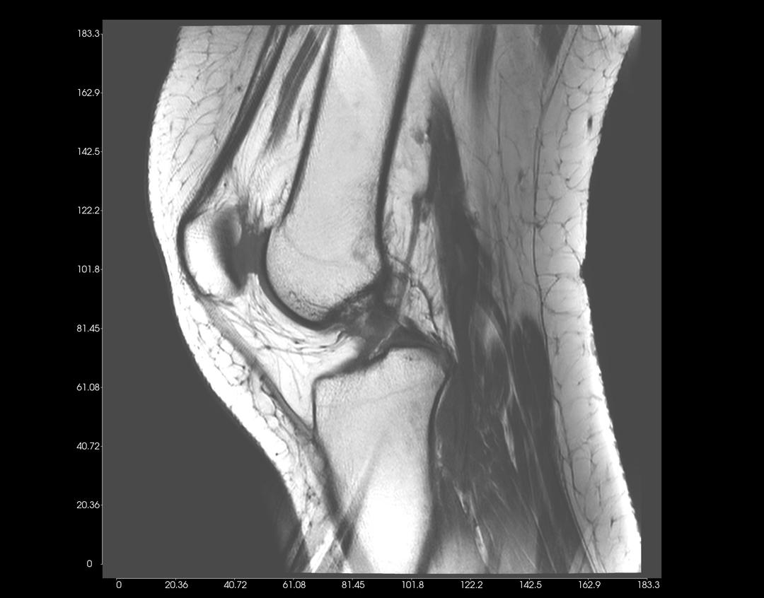
Left-click on an image, and drag upwards to increase contrast. Conversely, drag downwards to decrease contrast.
Click on the scroll wheel (mouse) and drag (pan) the image to where you want to place the image on the window.
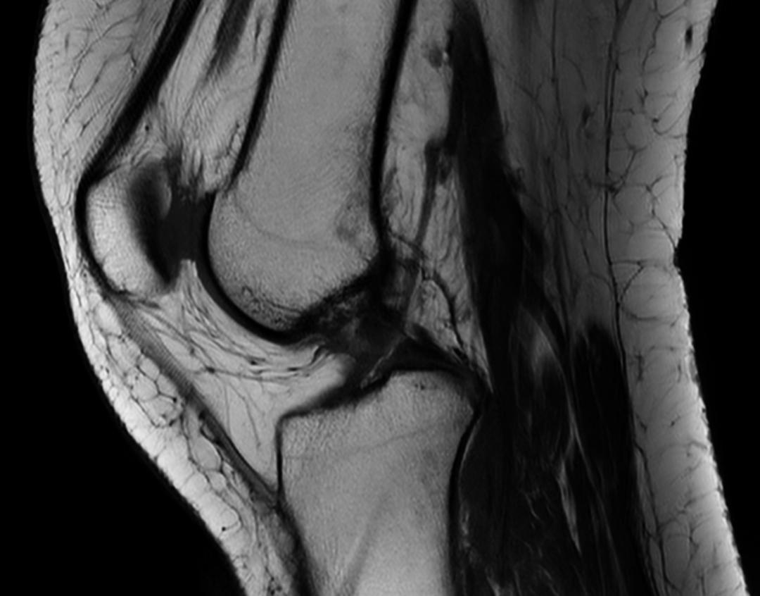
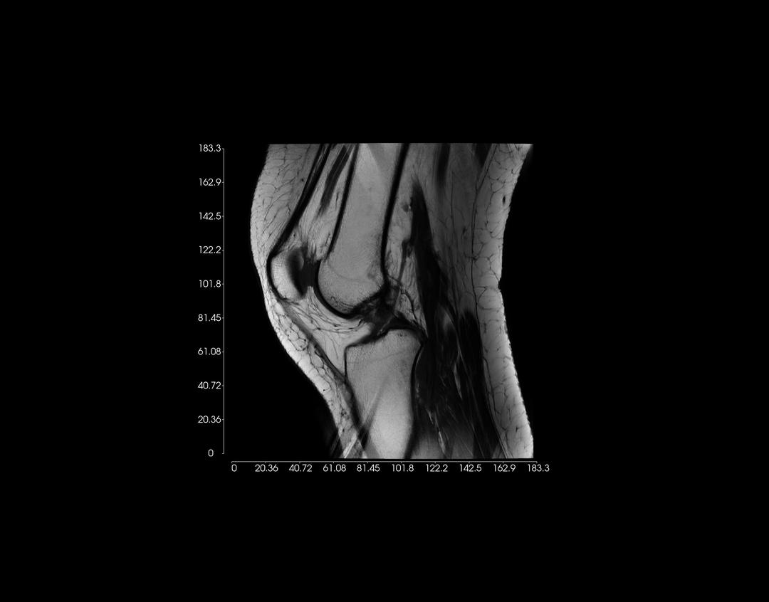
Right-click on an image, and drag upwards to zoom in. Conversely, drag downwards to zoom out.
Apply Colormaps
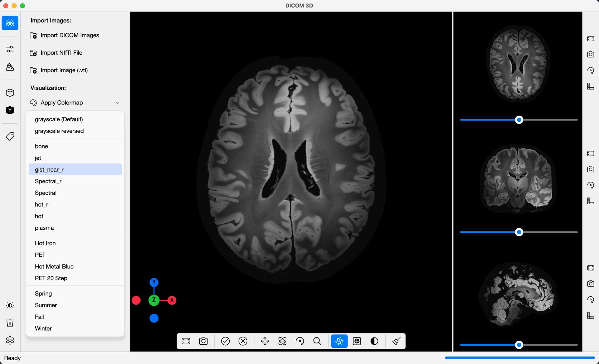
In the command bar, you will find the option to apply distinct colormaps to the imported images, for better visualisation. To apply one, simply click the Apply Colormap button, and select one of the options provided in the dropdown menu.
The colormaps come in two categories:
- Perceptually Uniform Colormaps
- DICOM Standard Colour Palettes
The DICOM Standard Colour Palettes include:
- Hot Iron: The Hot Iron color palette is often used in nuclear medicine applications to make differences in signal intensity (counts) more apparent to the human observer.
- PET: The PET color palette is often used in PET applications to pseudo-color the superimposed PET images when displayed fused with underlying CT images.
- Hot Metal Blue: The Hot Metal Blue colour palette is often used in nuclear medicine or PET applications to make differences in signal intensity (counts) more apparent to the human observer.
- PET 20 Step: The PET 20 Step colour palette is often used in PET applications to make differences in signal intensity (counts) more apparent to the human observer.
- Spring, Summer, Fall & Winter: These Colour Palettes are suggested for use in colour fMRI activation maps. They shade from one pastel colour to another which is distinctly different, making them suitable for illustrating either unipolar or bipolar activation. They convey activation strength within one statistical parametric map, while making it possible for the human observer to distinguish between different fMRI activation maps in the same blended display.
Learn more about the DICOM Standard Colour Palettes here.
In the example above, the gist_cnar_r colormap was applied.
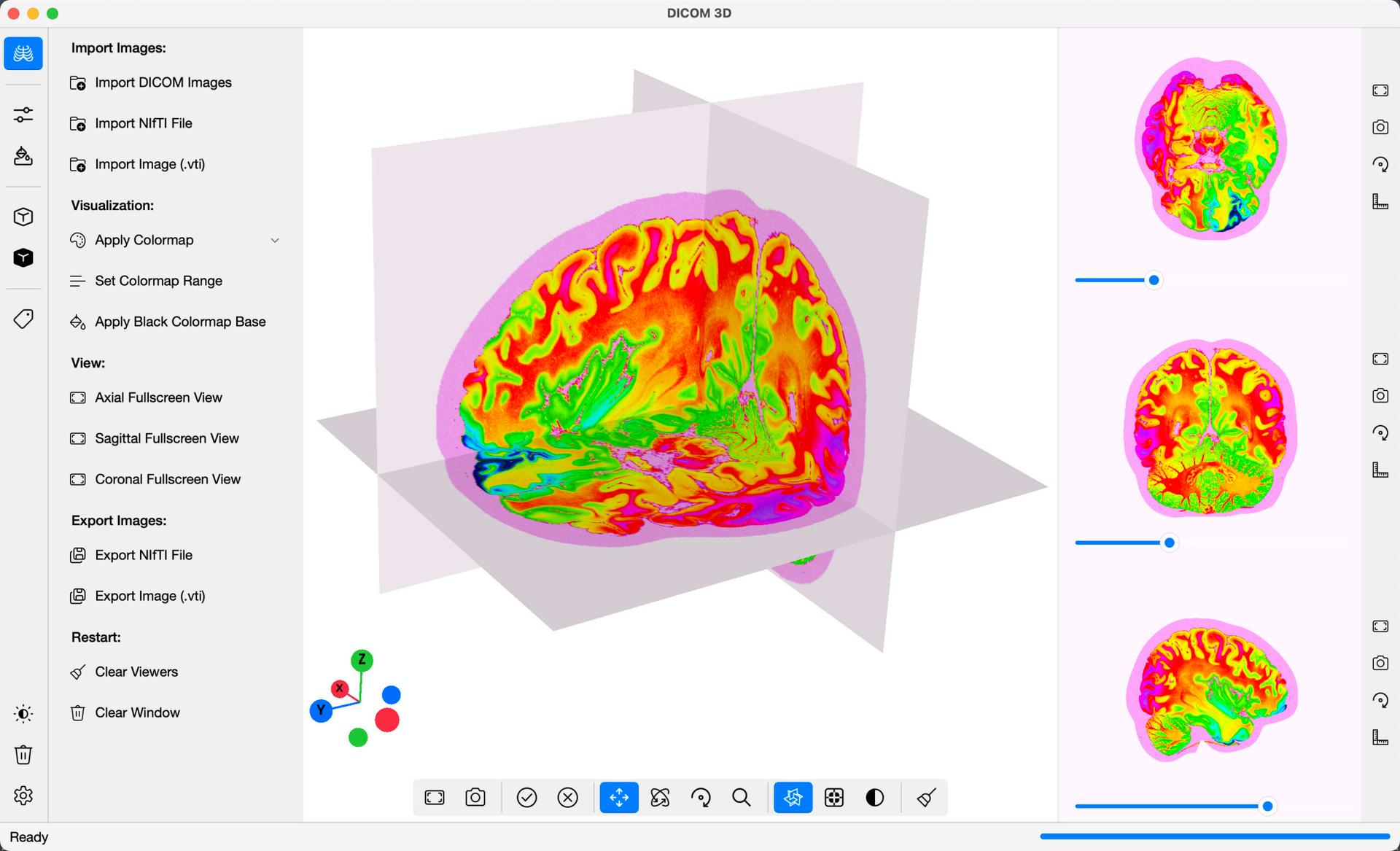
Colormaps can be further customised in two ways:
- Set Colormap Range: The Colormap Range value affects the ratio of values that the colormap is applied on. For the example above, a range of 0.90 was set, meaning that from the entire range of values/units in the DICOM Images, the middle 90% are visualized in the display, i.e. the lowest 5% and highest 5% of values are ignored.
- Apply Black Colormap Base: When active, this option ensures that the least value/unit in the Imported Images is assigned a black color, irrespective of the colormap applied. For example, in CT Images, the least Hounsfield Unit is -1024 representing Air. When active, this ensures that Air is visualised in black, irrespective of the colormap applied. Try this option with the jet colormap, whose base value is blue, to see its effects in action.
Import/Export NIfTI Files
The Neuroimaging Informatics Technology Initiative (NIfTI) is an open file format commonly used to store brain imaging data obtained using Magnetic Resonance Imaging methods. The NIfTI standard was specifically designed to address challenges in the neuroimaging field, focusing on functional magnetic resonance imaging (fMRI).
One of the main differences between DICOM and NIfTI, is that with NIfTI files, images and other data is stored in a 3D format. On the other hand, DICOM image files and the associated data are made up of 2D slices.
As NIfTI stores images in 3D Format, files can be easier to manage as an entire study is stored in one file, usually with the .nii or .nii.gz extensions. Compare this with DICOM Images, where a series of individual images/slices are stored in a folder, and not always in the correct order and orientation.
DICOM 3D features a NIfTI reader and writer, enabling users to work with NIfTI files as well as DICOM files, depending on preference.
3D Image Format (.vti)
DICOM 3D can also import & export DICOM Images in the 3D Image Format (.vti). This format can store an entire DICOM series in a single file. In addition, when exported from DICOM 3D, the .vti file will include the DICOM Tags. When imported, these tags will be added onto the DICOM Tags table. This format provides a much easier tool to store and share DICOM Series, as it is a single file, rather than a folder containing a series of images.
The Import Image & Export Image options can be found in the Visualize DICOM Images -> command bar , or on the menu bar, in the File Menu.
DICOM Tags
On the navigation bar (left), select DICOM Tags to bring up the DICOM Tags table. Upon importation of DICOM Images, the corresponding tags will be added onto this table. Scroll through the extensive list to get in-depth detail on the images in view.
Threshold Segmentation
This section covers the process of creating 3D Models from DICOM Images, based on threshold segmentation. With regards to DICOM Images, Image Segmentation can be defined as the process of partitioning a digital image into multiple image regions, based on certain criteria that make the image more meaningful and easier to analyze. In this context, threshold segmentation refers to the process of partitioning DICOM Images into regions of interest based on a particular tissue type.
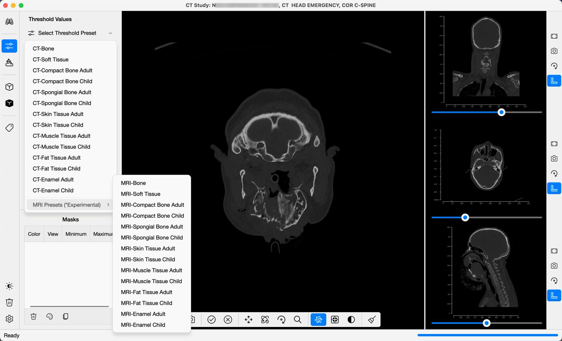
From the navigation bar, select Threshold Segmentation to launch the command bar, that includes the threshold segmentation functions. In DICOM 3D, a set of predefined threshold values are provided, that give you a basis from which you may refine your segmentation of the images. A list of industry standard CT threshold values are included for different body tissues, and a list of experimental MRI threshold values are included. For each preset, a minimum and maximum threshold value are defined. Values in the DICOM Images that fall between these two values are included in the image segmentation, whereas values that fall outside the threshold are excluded.
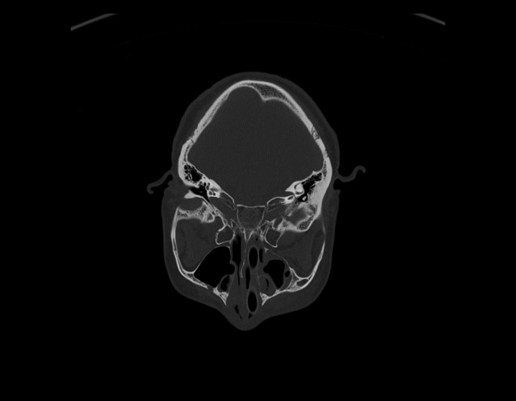
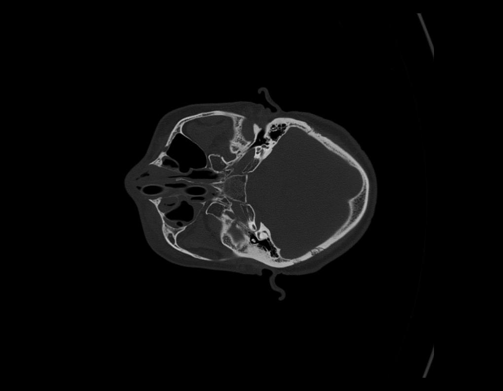
CT Scan Images are comprised of values referred to as Hounsfield Units. Hounsfield units (HU) are a dimensionless unit universally used in Computed Tomography (CT) scanning to express CT numbers in a standardized and convenient form. These units are named after Sir Godfrey N Hounsfield (1919-2004), a Nobel Prize winner who pioneered the CT scanner and made great contributions to radiology and medicine.
Generally, CT Images store values ranging from -1024 HU to 3071 HU; with -1024 HU representing air (in the lungs), 0 HU representing water and 3071 HU representing the most dense human tissue (Tooth Enamel). Metal medical implants generally have very high densities, and are attributed the highest value in the HU Scale, 3071.
From a visual perspective, when you first import DICOM Images into the application, they are displayed in grayscale, where -1024 HU is black and 3071 HU is white. The values in between are visualised in colours graduating from black to white in a linear manner.
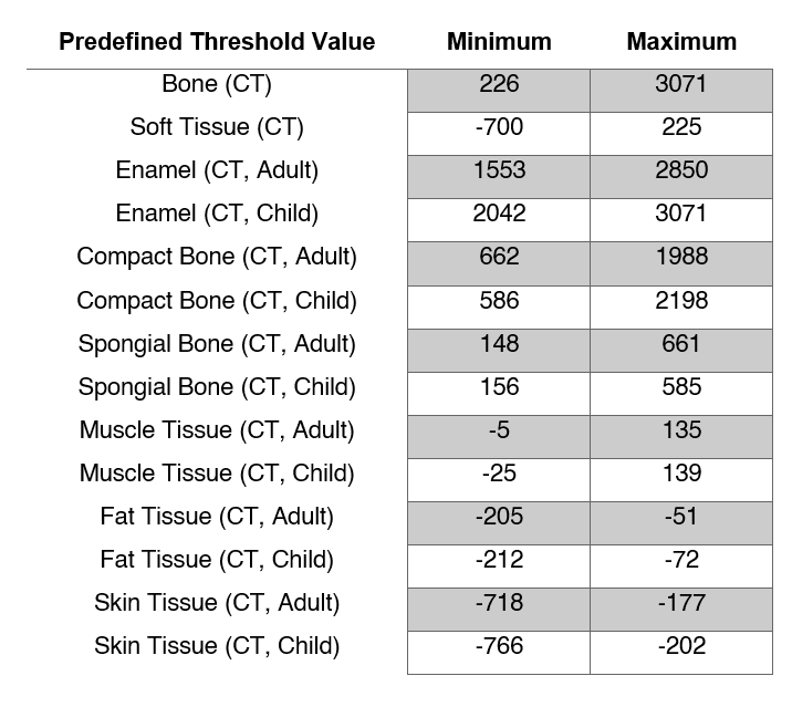
The table below summarizes the preset threshold values.
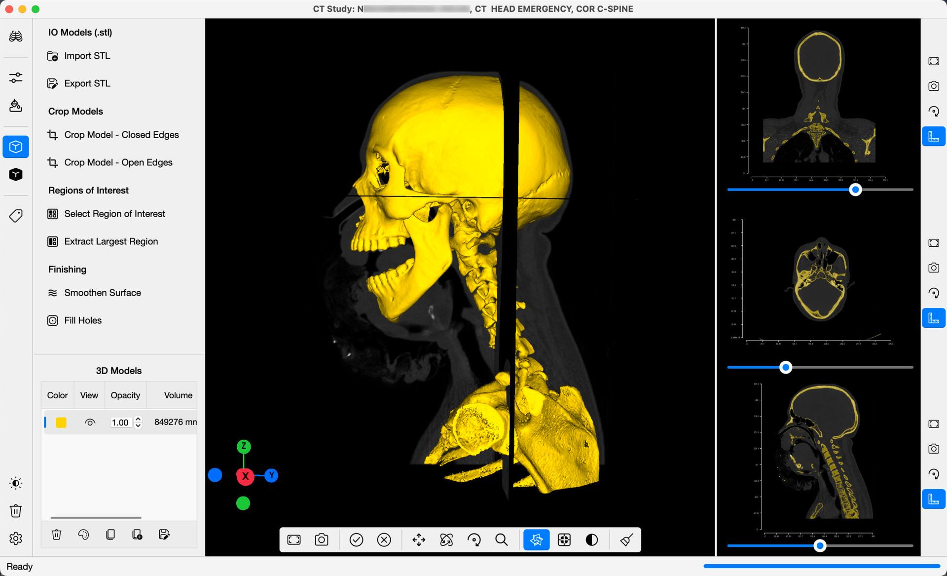
For this example, we will select CT-Bone from the dropdown menu. The minimum threshold value will be set to 226, and the maximum set to 2976. On the command bar, select Segment Images . A golden-yellow overlay will be added onto the DICOM Slices as in the image below, highlighting regions in the images representing bone tissue. In addition, a 3D Mask will be generated on the 3D View, providing a preview of what a final 3D Model may look like. You can manually edit the minimum and maximum values on the command bar, to refine your segmentation further.
Once you are happy with the segmentation, select Generate 3D Model , to create a 3D Isosurface Model derived from the DICOM Images. The 3D Slices can be added onto the 3D Viewer, as in the image below, by toggling on/off the 3D Slices button found adjacent to the viewer. The surface model can be refined further in the 3D Reconstruction command bar. The 3D Model can be clipped, individual parts selected, the surface finished, and more. This model can be exported in STL Format, to share with your colleagues, or for 3D Printing.
Below the Threshold Segmentation functions in the command bar, you will find a Masks Table. You will find 3D masks created from segmentation process listed here. The table includes options for editing or deleting generated masks.
Watershed Segmentation
This section covers the process of creating 3D Models from DICOM Images, based on watershed segmentation. The watershed is a classical algorithm used for segmentation. Starting from user-defined markers, the watershed algorithm treats pixels values as a local topography (elevation). The algorithm floods basins from the markers until basins attributed to different markers meet on watershed lines.
In this context, you (the user), mark areas in the DICOM Images that you want included in the segmentation, and mark the areas that you want excluded. These markers are in the form of seedpoints, that are placed on the slices in view. The algorithm then takes in these seedpoints, and calculates a segmentation of the imported images. This process is explained in more detail below.
From the navigation bar, select Watershed Segmentation to launch the command bar, that includes the watershed segmentation functions. Once you have the DICOM Images imported, on the command bar, toggle the Place Seedpoints switch on. When this switch is turned on, seed points can be placed on any slice in all 3 orientations. When turned off, the seedpoints are erased. Once turned on, two types of seedpoints can be placed:
- Foreground (Green): mark areas that you want included in the final model.
- Background (Red): mark areas that you want excluded from the final model.
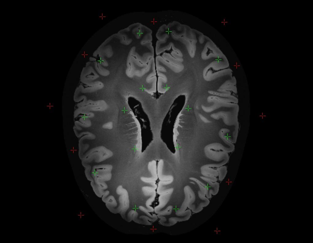
Activate either Foreground or Background on the command bar. Proceed to place the seedpoints on the DICOM Slices in view, as in the example below. The seedpoints can be placed on slices in all 3 orientations, to provide the algorithm with more markers to work from. In the example below, only the active slice in the Axial view was marked. Using your judgement, place enough seedpoints around the image to give the algorithm sufficient markers to differentiate between the two areas. You can delete the last seedpoint you placed, or delete all seedpoints, using the respective buttons on the command bar. Once you are satisfied with the markers, select Segment Images, and the watershed segmentation process will begin.
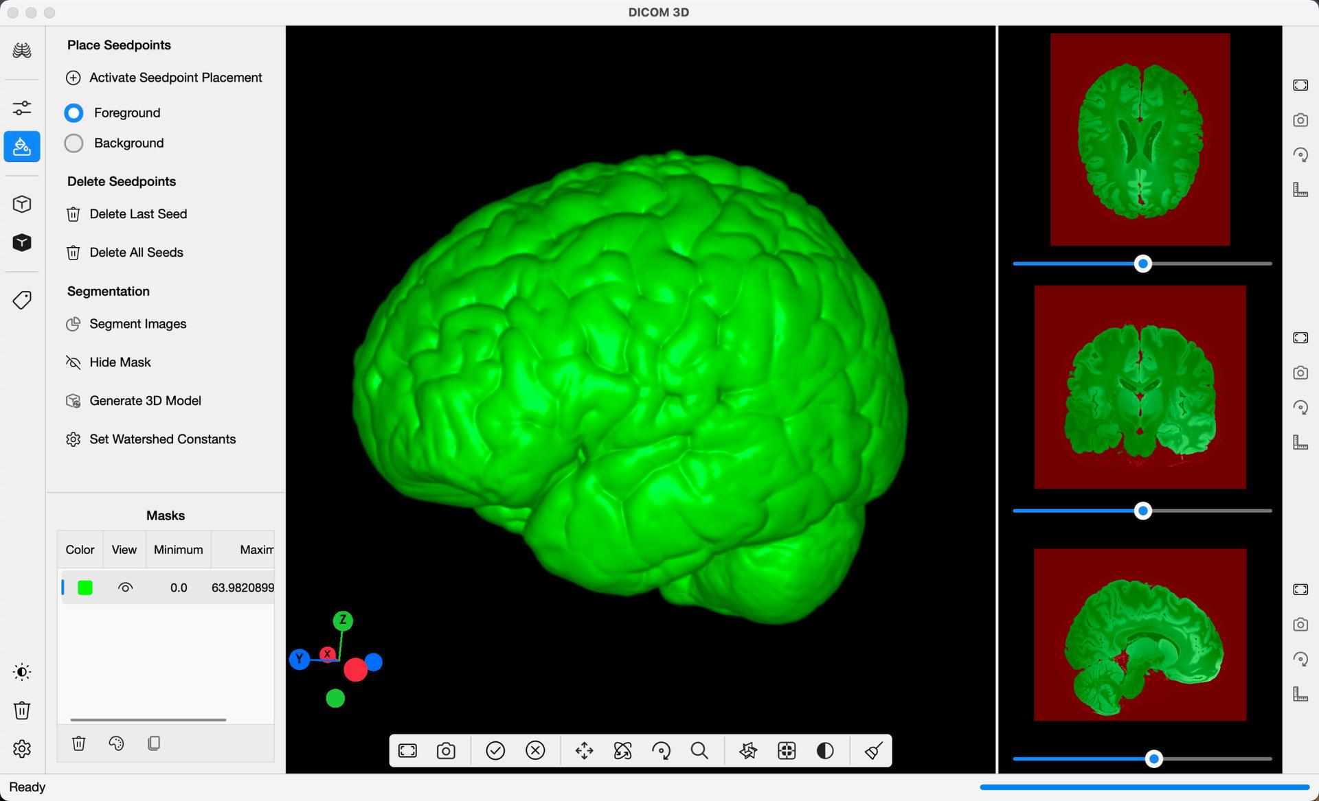
Upon completion, the algorithm will partition the Images into the two regions you marked. A mask overlay will be generated over the Slices, as in the example below, showing you the results of the segmentation. Scroll through the images to see the results. If you identify errors, or areas for improvement, use the Hide Mask button in the command bar to hide the mask overlay, and place more seedpoints on the Images. Repeat this process until you are happy with the final results.
In addition to a mask overlay placed on the DICOM Images, a 3D Mask will be generated on the 3D Viewer, providing a preview of what a final 3D Model may look like. Select Generate 3D Model, to create a 3D Isosurface Model derived from the segmentation. This model can be edited further from the 3D Reconstruction command bar, launched by selected 3D Reconstruction in the Navigation Bar.
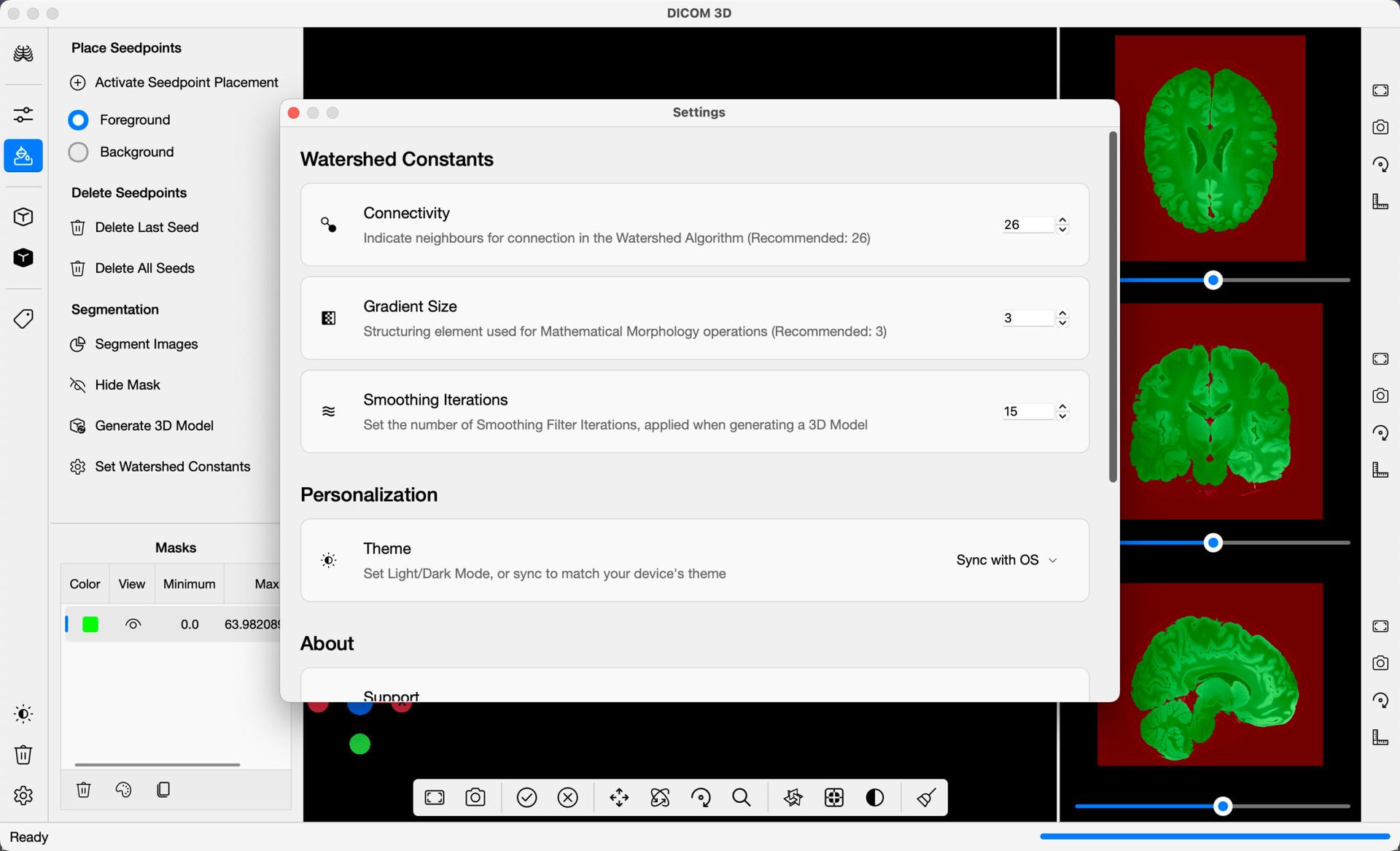
The following parameters can be adjusted from the application Settings, to further refine the watershed algorithm to your liking:
- Connectivity: Indicate neighbours for connection in the watershed algorithm.
- Gradient Size: Structural element used for Mathematical Morphology operations, before the watershed algorithm is applied.
- Smoothing Iterations: Set the number of smoothing filter iterations applied, when generating a 3D Model.
Threshold vs Watershed
While both thresholding and watershed segmentation can be used on both CT and MRI Images, each method has its strengths and weaknesses.
Thresholding
Strengths
- Excellent with CT Scans. The preset thresholding values provided for different tissue types, give great segmentation results with CT Images.
- Speed. Thresholding doesn't require extensive input from the user, and a study can go from importing images to final 3D Models in a couple of minutes.
Weaknesses
- Control. Thresholding doesn't provide the user with a lot of control of the segmentation process. Each part of the image that matches a threshold value is picked out, even if it is in areas that the user doesn't want. These areas would have to be excluded in the final 3D Model.
- MRI Scans. While experimental preset thresholding values have been provided for MRI Scans, these values do not always work well, and segmentation can be frustrating.
Watershed
Strengths
- Control. This method provides complete control over the segmentation process. As the user can manually pick out areas that they want excluded from the final model, the user can dictate the make-up of the final 3D model.
- Good with CT and MRI Scans. Watershed segmentation works great with both MRI and CT scans, providing a universal segmentation method.
Weaknesses
- Can be time-consuming. With greater control and more user input, more time is spent refining the segmentation. If the area you want to pick out is very specific, or the image data provided is noisy, the watershed segmentation can take more time than expected for you to end up with a model that you are happy with.
Conclusion
All together, thresholding and watershed segmentation provide a comprehensive set of image segmentation methods that can be used on almost any case. Based on the strengths and weaknesses above, you can choose the method best suited to your needs. Alternatively, you can try both and see which method produces the best results.
Cropping
DICOM 3D features a simple widget that allows you to crop 3D models with relative ease. Once a 3D Surface Model is loaded into the 3D Viewer, select Crop Model - Closed Edges on the command bar.
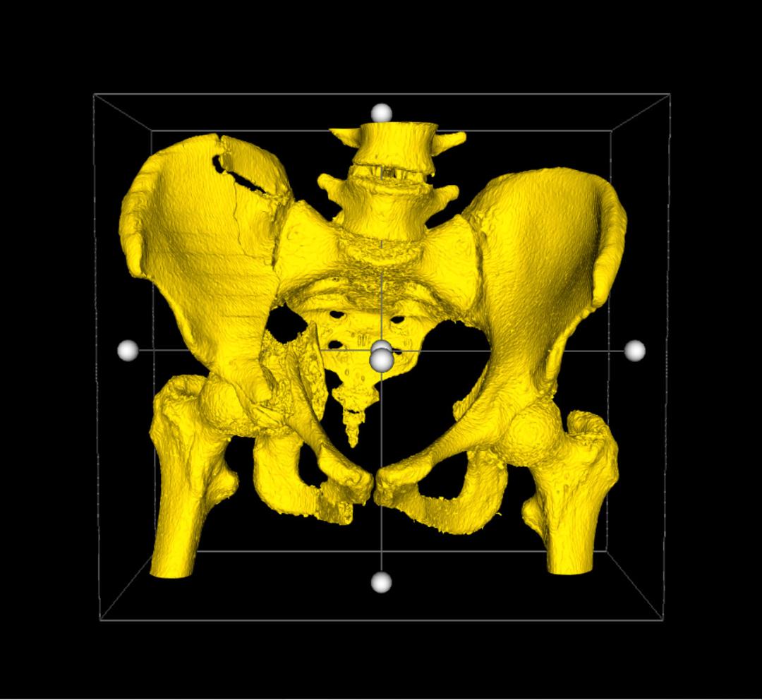
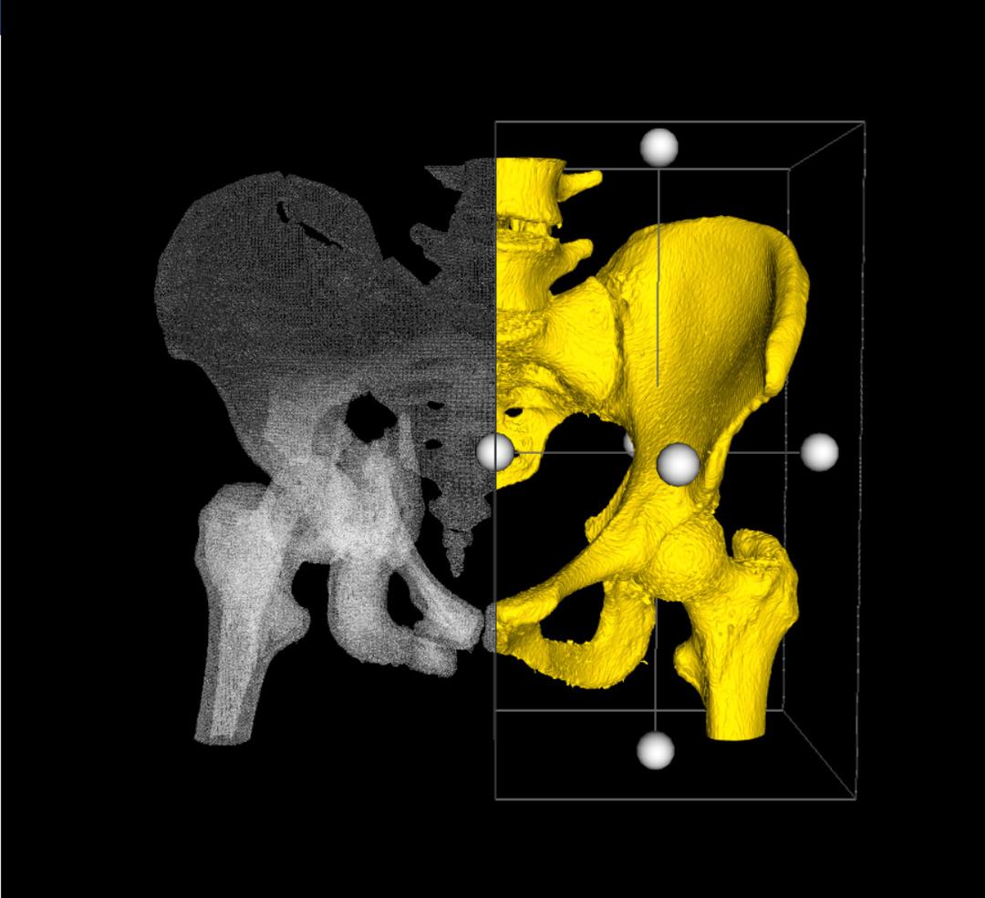
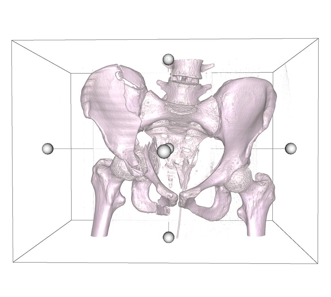
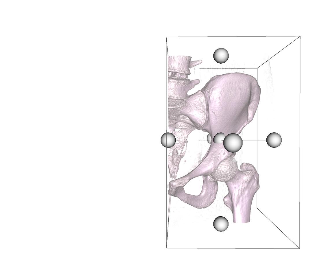
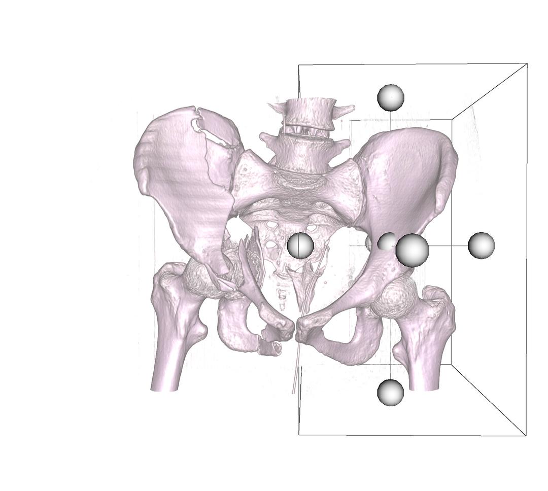
This will add a bounding box around the 3D Model in view. Each face has a handle (sphere), which you can select and drag inwards to crop the model along that axis. On release of the handle, the cut will be performed. As you drag any face of the bounding box inward, a preview of what remains and what is cropped out is generated in real-time. Take the example of a pelvic fracture below.
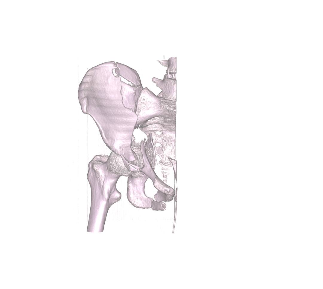
Once you are satisfied with the preview, simply select the Accept button, highlighted in green to the right of the 3D Viewer, and the crop will be performed. If you wish to undo the operation, simply drag the handle back to its original position. If you want to undo the operation, and disable the crop widget altogether, select the Cancel button, highlighted in red to the right of the 3D Viewer.
Difference Between Crop Model - Closed Edges, and Crop Model - Open Edges
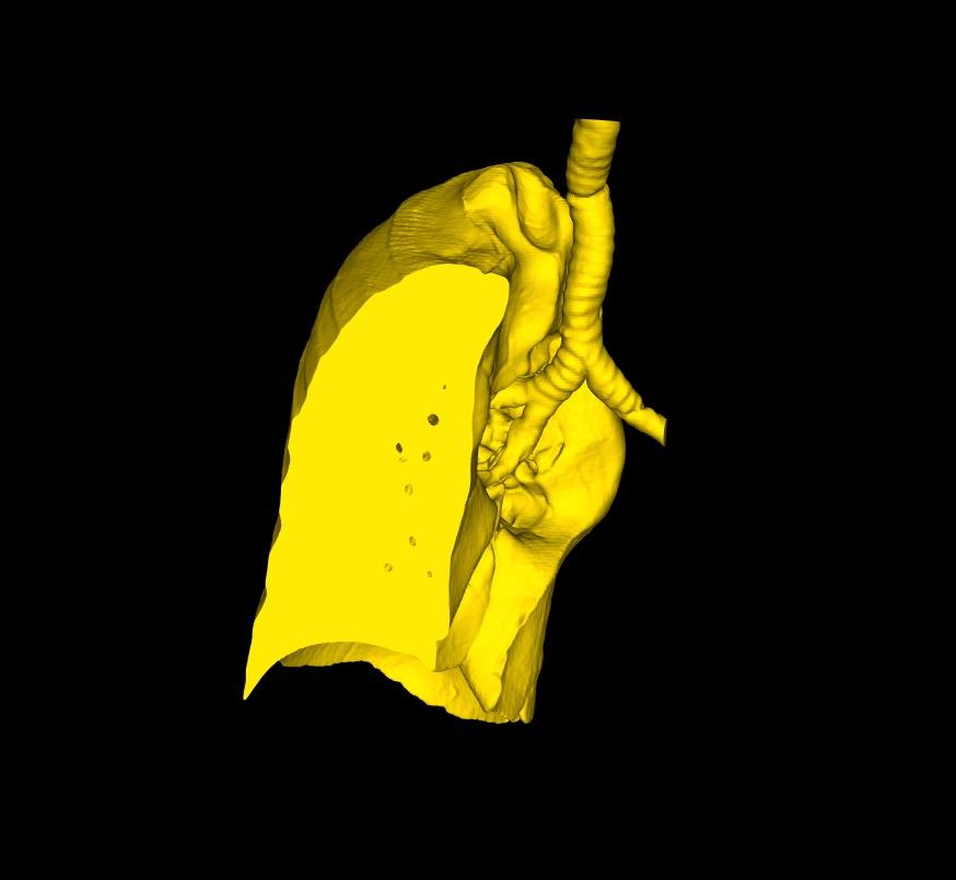
On the command bar, you will notice the two buttons above. The main difference between the two functions, is what happens to the clipped surface after the cut. With the first, the boundaries of the cropped model are automatically filled by a flat surface, thereby making the 3D Model watertight. With the second, the boundaries are left open as illustrated below (right).
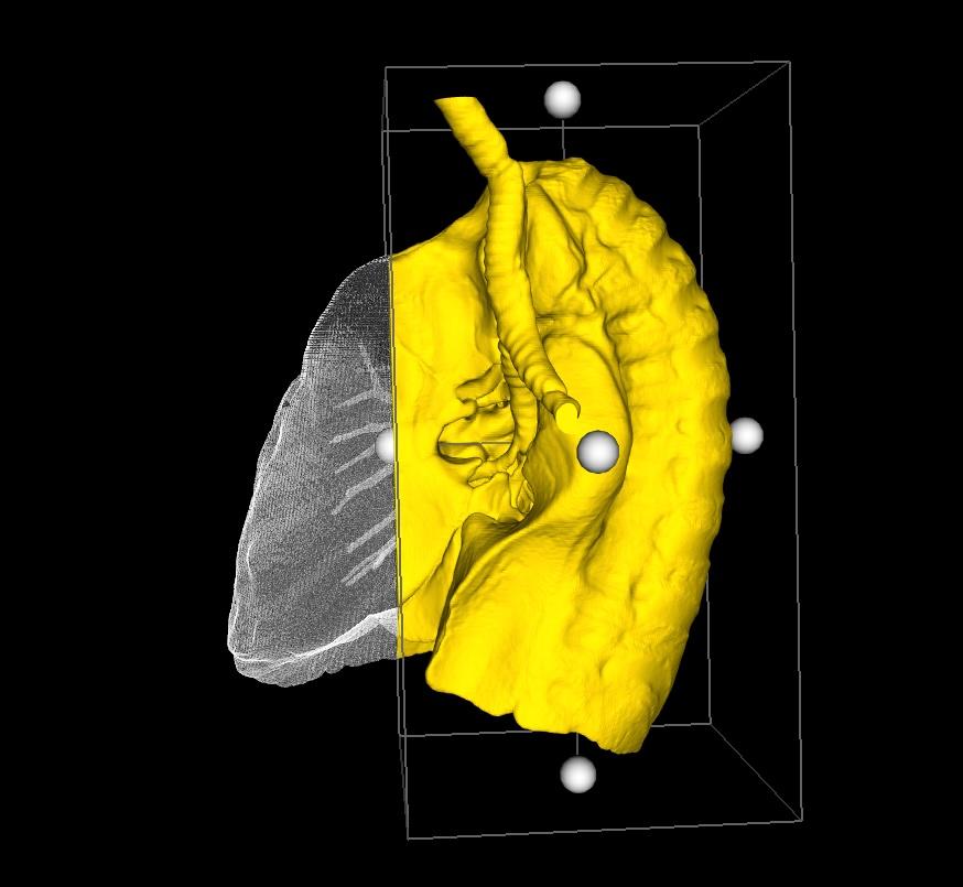
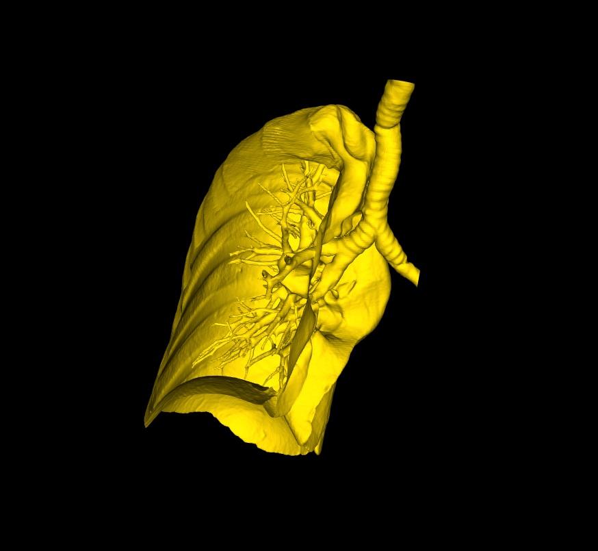
Closed Edges: Useful if you want to view internal structures found within a closed surface.
Open Edges: Useful in most other situations; particularly if you want to export the model to create a physical model, by 3D printing for example.
Regions of Interest
Frequently, you will generate a 3D model that consists of more parts than you want to focus on. For example, if a CT Scan covers the whole chest, but you are only interested in a particular body tissue or organ. In order to narrow down to the parts that your after, you have two options: crop the model using the crop tools, or, use the Regions of Interest Functions.
Extract Largest Connected Surface
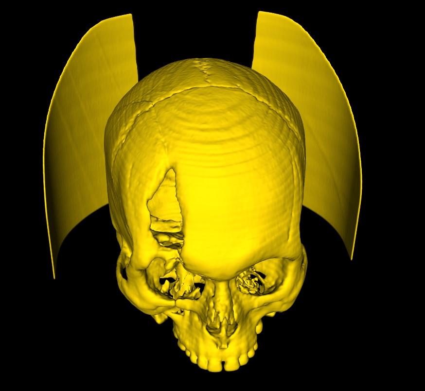
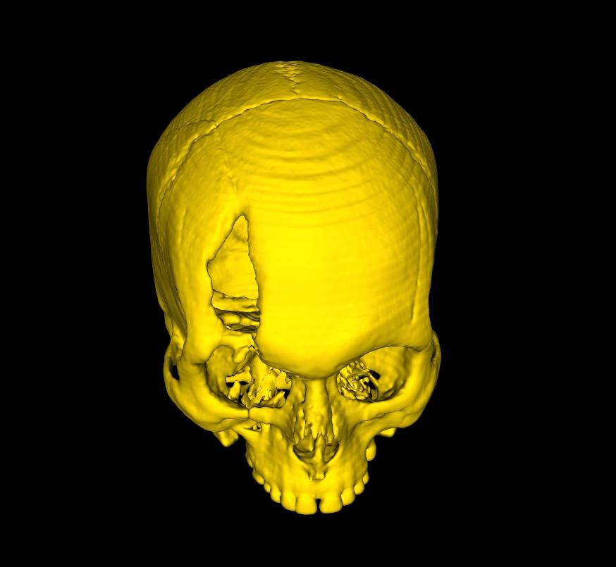
Take a head scan for example. A generated model of the cranium may often contain the head rest/support used during the CT Scan. Selecting the Extract Largest Region on the command bar, will automatically detect the largest individual surface in the model, and extract it, deleting all other disconnected parts. The same function can be used in cases where the generated 3D model contains multiple body tissues, of which you are only interested in the largest tissue. So long as the part you're interested in is disconnected from the rest, and is the largest single surface, this function is ideal.
Select Regions of Interest
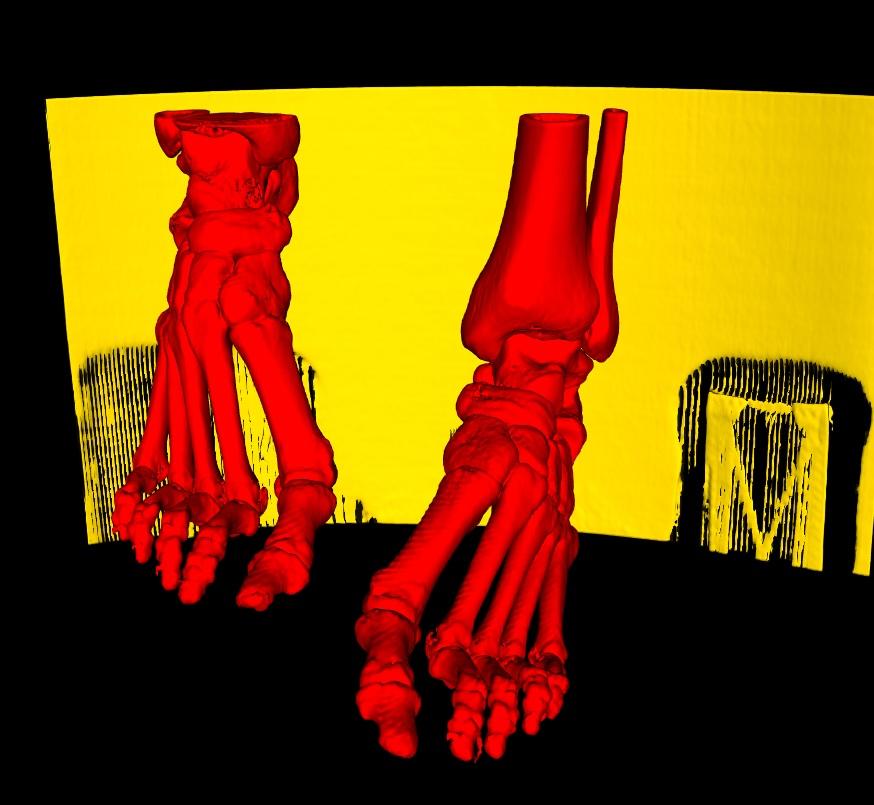
We will use a CT Scan of feet as an example here. An analysis of the feet bone structure, would yield a generated 3D model as below. Here, if you're interested in extracting both feet, you would use the Regions of Interest Button. The button activates a function, that detects all disconnected parts. Once done, you would simply need to select (left-click) on each part that you wish to keep. Conversely, if you accidentally select a part that you wish to de-select, simply right-click on that part. Any selection is adjusted to red.
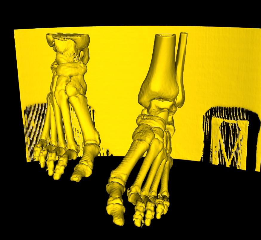
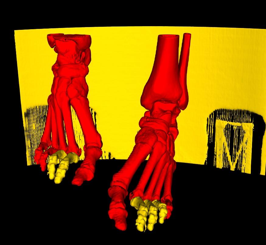
If any smaller parts turn out to be disconnected in the 3D Model, as for the toes on each foot still in yellow, simply continue to select each of the individual parts until all regions that you are interested in have been selected.
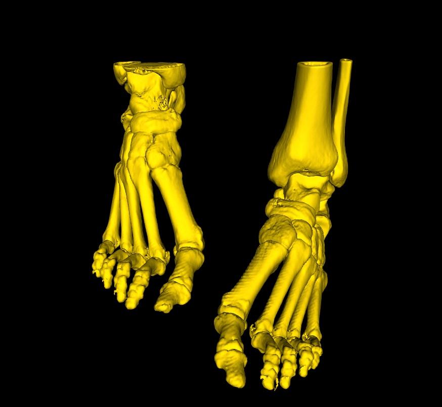
Finally, once you are satisfied; select the Accept button to extract your selections, or Cancel, to restore your original model.
Apply Medical Color Presets
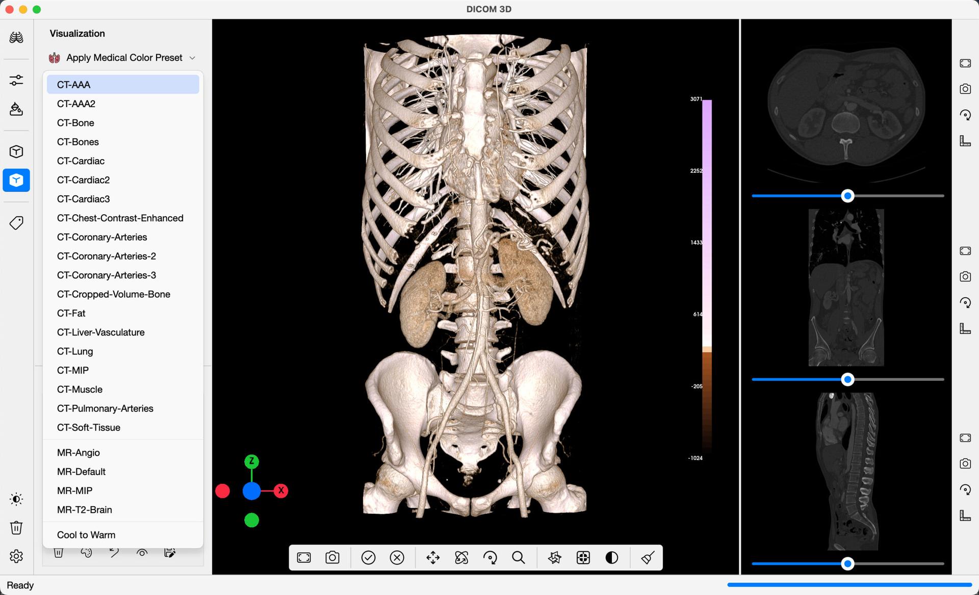
Once DICOM Images are imported, select an option from the Apply Medical Color Preset dropdown menu, to gain a quick 3D view of the loaded images in a more realistic color structure. Color presets for the CT & MRI Modalities are provided. Choose the option that best fits your region of interest.
A good start for CT images would be CT-AAA or CT-AAA2 presets. Either of these presets would provide a general preview of the 3D Image. For MRI Images, the MRI-Default preset would provide a great general preview of the 3D Image.
In the example below, the CT-AAA preset was applied. A Scalarbar is added to the right of the window, which gives a representation of the colormap applied to the Image, along with Intensity Values where the colour transitions are applied.
An orientation widget is also added onto the 3D Viewer, which includes handles in the X, Y and Z directions of the image. Select any of the handles, for a view of the Volume in the direction selected.
Customizing Medical Color Presets
Each colormap includes a list of colour values (RGB), opacity values, and the intensity values (Hounsfield Units for CT) whereby each colour - opacity pair is applied. The Volume Color Properties table, located on the bottom right of the DICOM 3D window, is populated with these values, once a preset is applied. It is from this table that the colors can be customized. Adjustments to the active preset can be made as follows:
- Color: You may change the color at each point by clicking on the palette icon below the table, and choosing one from the resulting color picker.
- Opacity: Adjust the opacity at a specific point, with the spinbox arrows. You can also type in the value directly. The values range from 0 to 1, and must include two decimal places.
- Value: Adjust the intensity value in the same way as the opacity. The values range from the minimum to maximum intensity values found in the imported dicom images.
Each adjustment will be updated instantly on the 3D Viewer. If you are unhappy with any changes applied, select the reset icon below the table. This will clear any adjustments, and restore the original preset.
Cropping Volumes
DICOM 3D includes a cropping widget that allows you to clip the volume to a particular region of interest. Select Crop Volume to activate this widget. Once activated, a bounding box is added onto the volume, with a handle on each face.
Select a handle and drag inwards to specify the region where the crop function is executed. You can also select any face on the cube, and rotate the widget. This gives you flexibility to specify the region you want clipped, in all directions. Once satisfied, select the Accept button to perform the cut, or Cancel button to restore the volume.
Crop Volume - Inverted
As the name describes, this option works in reverse to how the crop volume function works. In this case, the region specified by the cube widget is clipped, and not kept. This difference is illustrated when the two images above, are compared to the process highlighted in the two images below.
Import & Export of Volumes
DICOM 3D includes the option of saving a 3D Volume Render for later. You may export the render to your device and share with colleagues, or import later. This is especially useful when you have customized a Medical Color Preset, to a degree that you are very happy with, and don't want to have to recreate the Volume Render every time you load the same DICOM series.
The Volume is exported in the same 3D Image Format (.vti) described in Section 3.6 above, under DICOM Visualisation. However, this time, the active medical color preset at save is included in the .vti file. This .vti file can be loaded onto other Medical Imaging software, but will not visualize the Volume Render, only the DICOM Images. The Volume Render saved on the .vti file can only be displayed on DICOM 3D.
Theme
DICOM 3D features a fully integrated Dark Mode, that can be activated at any time. This can be set in three ways: from the Toggle Light/Dark Mode button on the Navigation Bar, from the Theme menu in the menu bar, or in the application Settings.
Alternatively, there is the Sync to OS option, that matches your device's theme at all times. This is selected by default.