In Vista, you can quickly visualize volumes either through application of 3D Scientific Colormaps or Medical Color Presets. Of the two, application of volumetric scientific colormaps is more versatile and dynamic, allowing you to customize the volume render to highlight your specific regions of interest with relative ease. Unlike Medical Color Presets, which consist of predefined values that may or may not fit your image data well, the Colormaps are applied dynamically to your data, able to fit images with a wide or small range of values with little compromise.

Follow the guide below to understand how it works, and how you can customize the volume render with the Colormap Widget to achieve the best results.

How It Works

Click on the 'Select Colormap' dropdown menu, and select any of the colormaps in the list, to apply a colormap to the volume. In a few seconds, a volume render of your image data will appear on the Canvas. The volume will exhibit the range of colors in the chosen colormap. You can interact with the model as described in the Interaction Section.

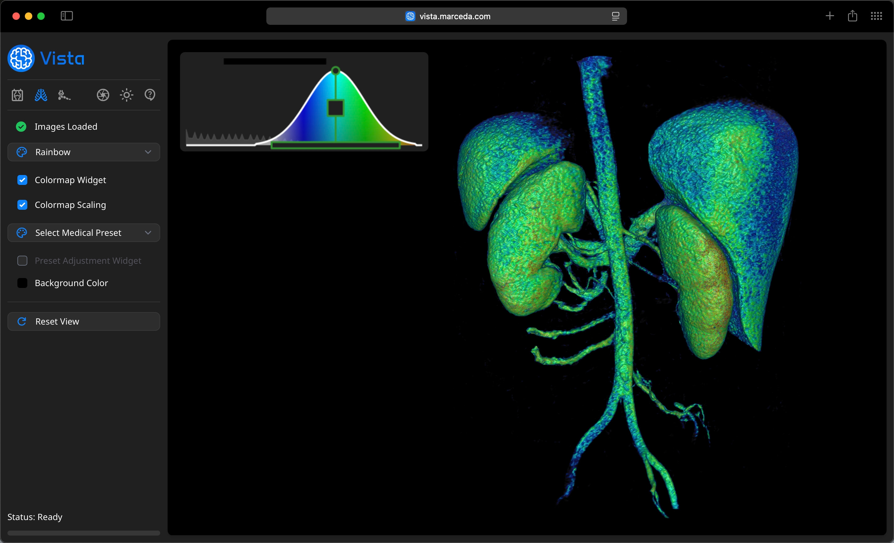
In the example above, the 'Rainbow' colormap was selected. The volume rendering works through application of Gaussian Functions. In this context, a Gaussian function is a mathematical representation used to model the opacity of values in the image dataset. So, for every color defined in the colormap, a corresponding opacity value is assigned based on the Gaussian function. This function is characterized by its bell-shaped curve, defined by its mean (or center), height (maximum value), width (spread), and biases, which can adjust its shape. Application of this function effectively allows for smooth transitions between transparent and opaque regions in the render.

Note the shape of the curve in the Colormap Widget to the top-left of the Canvas. This is a visual representation of the active Gaussian function in the volume render. The peak represents an opacity of 1, and the valleys on each side represent the declining opacity all the way to 0 (transparent). You can interact with this widget to manipulate the Gaussian function, and visually control how different values in a volume rendered, enhancing the visualization of complex datasets.

Customization

As described above, a Gaussian function has four main characteristics, each of which can be can be adjusted as below:

• Position: This parameter sets where on the range of image data values the Gaussian's peak occurs. For instance, if you specify a position of 50, it means that at this value, the opacity will be at its maximum (determined by height).
• Height: The height parameter determines how opaque that point will be. A height of 1 means full opacity at that scalar value, while lower values indicate varying degrees of transparency.
• Width: This parameter affects how quickly the opacity transitions from opaque to transparent as you move away from the peak position. A larger width results in a smoother transition, while a smaller width creates a sharper drop-off in opacity. As a result, this parameter also affects what data is visible on the volume render.
• Biases: These parameters allow for adjustments to the Gaussian's shape, enabling asymmetrical curves that can better fit more complex data distributions.

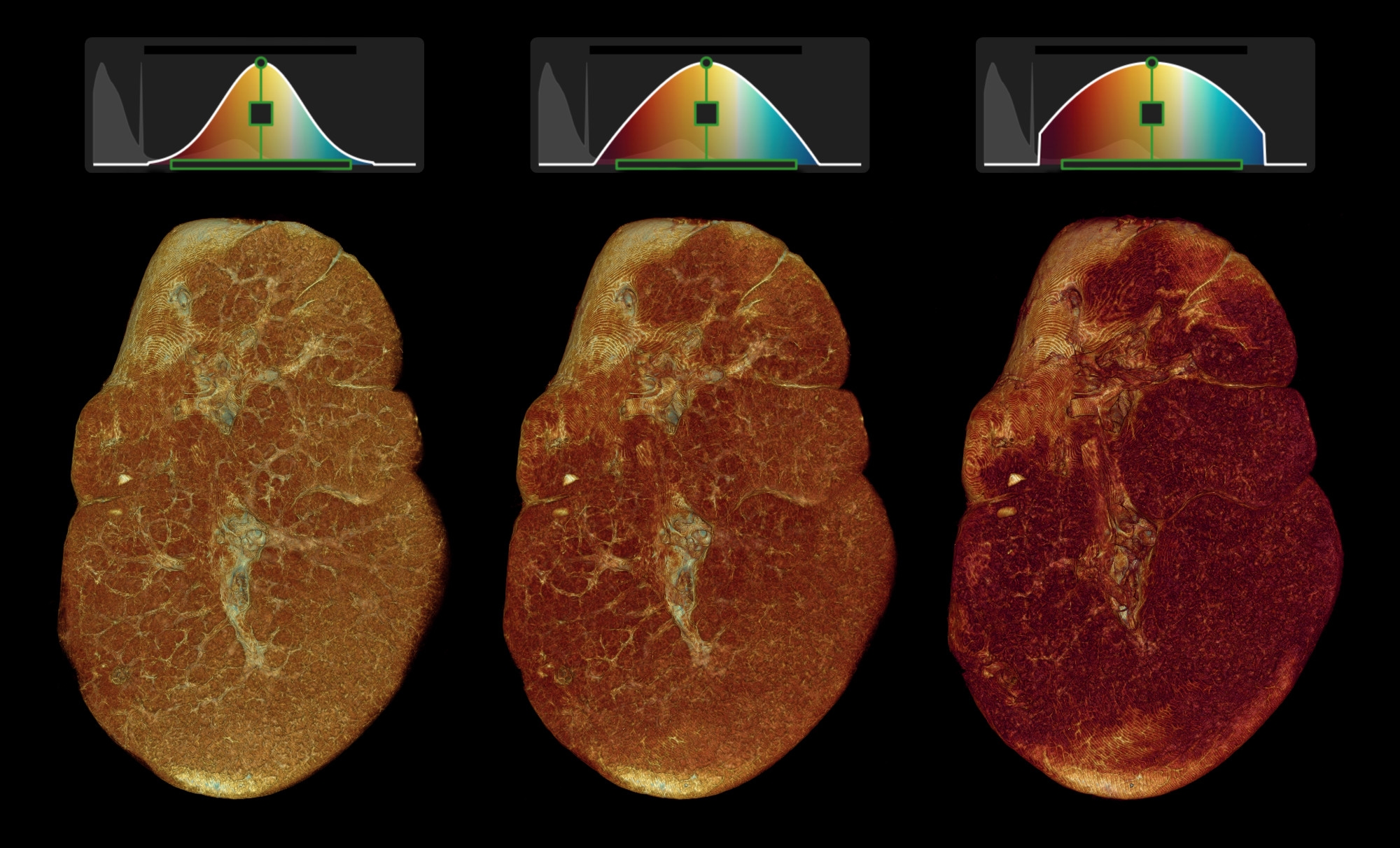
The examples above show a Gaussian function applied to image data of a Spleen, demonstrating how adjustment of opacity values can hide or reveal inner structures in an organ.

Observe the Colormap Widgets, each of the Gaussian function parameters can be identified: the peak (circle at the top), position (vertical line in the middle of the bell-curve), width (narrow rectangular base at the bottom), and biases (controlled using the square in the middle). All are highlighted in green. Adjust these parameters as follows:

• Peak: Left-Click on the circle, and drag downwards to reduce or drag upwards to increase the maximum opacity.
• Position: Hover over the curve until you see the cursor change to a hand icon (outside the circle, square and base). Left-Click to grab the position, and drag left or right to select the midpoint of the curve.
• Width: Left-Click on the narrow rectangular base on the bottom of the curve, and drag right to increase or left to decrease the width of values included in the volume render.
• Biases: Left-Click on the square in the middle, and drag left or right to adjust the x and y biases of the Gaussian function.

The 'Colormap Widget' is fully functional on touchscreens, and is fully compatible with touch gestures.

You can further customize your volume render, by adding multiple Gaussian functions. This can be particularly useful when visualizing complex datasets. Simply double click at any point on the widget to add a Gaussian function. Conversely, Right-Click on any curve, to remove the active Gaussian at that point.

Colormap Scaling

There is one other method of customizing the application of colormaps in this context. By default, the colormaps are scaled to fit in the width of the active Gaussian function(s). This allows the full spectrum of the colormap to be applied to the range of values that you specify.

There may be instances where your focus is on a very small range of values, and application of the entire colormap will hinder the clarity of your volume render. In such cases, you can uncheck 'Colormap Scaling' in the Tools Sidebar. When disabled, the colormap will be applied evenly to the entire image dataset, irrespective of the width you set using the Colormap Widget.